Bioinformatic modelling of the impact of probiotic supplementation on microbiomes of breeding ponds and of digestive tract of the Common carp (Cyprinus carpio)
Title: Bioinformatic modelling of the impact of probiotic supplementation on microbiomes of breeding ponds and of digestive tract of the Common carp (Cyprinus carpio)
Key investigators: Joanna Szyda, Tomasz Suchocki, Anita Brzoza, Magda Mielczarek, Dawid Słomian, Michalina Jakimowicz
Students involved: Piotr Hajduk, Laura Jarosz, Marek Sztuka
Period of work: 2022-2026
Funded: National Science Centre
Introduction
In recent years, there is great interest in the use of effective microorganisms as probiotic supplementation in aquaculture to improve water quality, inhibit pathogens, and promote the growth of farmed fish. The use of probiotics, which control pathogens through a variety of mechanisms is viewed as an alternative to antibiotics and has become a major field in the development of aquaculture. Considering the potential benefits of adding probiotics, many farmers have recently been using commercially available products in their fish farms.
Although the practical efficacy of probiotic products in aquaculture has been extensively studied, there is a shortage of research related to practical, on-farm (i.e. not experimental) application of probiotic products in the Common carp (Cyprinus carpio) breeding. Especially when probiotics are implemented as a mixture of effective microorganism communities and not as a particular bacteria species.
This study aims to investigate the practical on-farm application of probiotics in Common carp (Cyprinus carpio) breeding, particularly when implemented as a mixture of effective microorganism communities. Probiotics have gained attention in aquaculture as an alternative to antibiotics, with the potential to improve water quality, inhibit pathogens, and promote fish growth. However, there is a lack of research on the practical application of probiotics in Common carp breeding. The study will assess the impact of probiotic supplementation on the water, sediment, and fish intestinal microbiota diversity in earthen ponds, which simulate practical fish breeding conditions. The study will also analyze the differences in water metatranscriptome compositions, with two major factors considered: (i) probiotic supplementation of water, and (ii) probiotic supplementation of feed. The findings of this study will contribute to the understanding of the practical application of probiotics in Common carp breeding and provide insights into the potential benefits of using probiotics in aquaculture.
Hypoteses
1. Microbiota diversity of water, sediment and fish intestinum can be altered by probiotic supplementation of water/feed.
2. Microbiota dynamics of water, sediment and fish intestinum differs between different probiotic supplements of water/feed.
3. There exists a correlation between the degree of microbiota diversity in water, sediment and in fish intestinum.
4. The abundance of particular taxonomical units does not change linearly in time.
5. Water metabolic activity expressed by water metatranscriptome varies between different probiotic supplements of water/feed.
Progress
The experimental part of the project was carried out during its first year at the Golysz experimental station, belonging to the Polish Academy of Sciences Institute of Ichthyobiology and Aquaculture. The complex of experimental aquaculture ponds comprised 32 equal-sized ponds of 600 m2 area. All ponds had individual water supply from the Vistula river, which guaranteed uniform physicochemical characteristics of supplied water. The whole experiment was carried out within one full fish production season. During the experiment, all ponds were stocked with the Common carp (Cyprinus carpio) hatchling applying a density of 30,000 larvae per hectare. Two most commonly commercially available probiotic water supplements, as well as one commercially available feed supplement, were tested in the experiment. The whole experimental setup involved 25 experimental ponds, from which 5 ponds were used as a control.


From each pond, 5 samples of water and sediment were collected 3 times during the experiment: (1) in the first month of the experiment, (2) after 2 months, and (3) in the last month of the experiment. In the last month of the experiment, fish intestinal samples were also collected from 5 individuals per pond, as well as one water sample per pond collected for metatranscriptome analysis. DNA was isolated and amplified for sequencing of selected hypervariable regions of the 16S rRNA gene from each sample intended for metagenomic analysis. Moreover, during the course of the experiment, regular measurements of water physicochemical parameters (temperature, pH, O2 concentration, nitrite, nitrate, ammonia, phosphorus) were performed to collect metadata describing water quality. At the beginning and the end of the experiment, sediment samples from all ponds were collected to analyze potential differences in sludge accumulation between ponds.


Sequencing
The sequencing process went well. The number of sequences for water samples can be found below.
Analysis
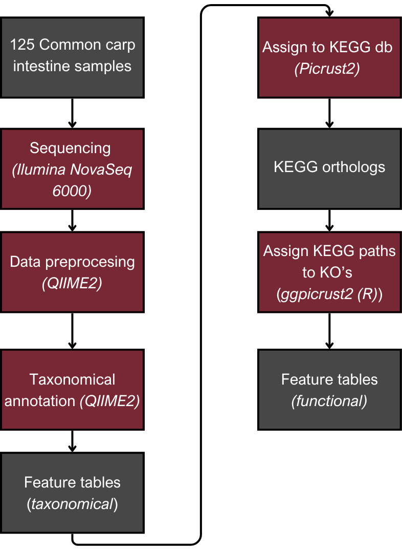
For the 16s RNA analysis, the QIIME2 software was used. First of all, adapter trimming eliminated non-biological information was done. A quality threshold of 30 was applied to exclude sequences with a quality score below that threshold. Moreover, sequences shorter than 200 nucleotides were removed. Paired ends were merged with specific thresholds, maintaining sequence length consistency within 16S regions. The denoising step was performed, which produced Amplicon Sequence Variants (ASVs), distinguishing single-nucleotide differing sequences—an advancement over Operational Taxonomic Unit (OTU) tables. These tables were then used to determine the microbial composition of the samples. After that taxonomic assignment was performed. The alpha diversity metric was computed based on the taxonomic assignment. Furthermore, ANCOM was employed to conduct a differential abundance test for detecting alterations in the microbial composition between experimental groups.
The next step was to assign the ASV to Kyoto Encyclopedia of Genes and Genomes (KEGG) pathways. To achieve this, we used pictrus2 software to assign ASV to Kegg orthologs (KO), then KOs were used as an input to ggpicrust2 library (in R) that assign pathways based on KO’s. The last step in this part was to check if there are significant differences in the abundance of KEGG pathways between different design setups; this was done using Deseq2 package in R.
Comparative Deep Learning architectures for Microbiome Classification
The model aimed to construct a neural network classifier using Keras under TensorFlow. The dataset consisted of feature tables representing the abundance of bacterial families in various individuals from different ponds. These tables were merged into a single dataset, including all bacterial families present in at least some individuals. Missing values were replaced with zeroes.
To differentiate microbiomes and classify individuals based on the probiotics they were fed, we tested and compared various deep learning methodologies. Specifically, we explored different dimensionality reduction techniques and model architectures to develop a deep learning classifier capable of performing this task.
For classification, the experimental setup (i.e., the type of probiotics fed to the individuals) was used as the class label, while the abundance of bacterial families served as predictors.
Accuracy was used as the primary evaluation metric. It was calculated on a binary basis, where each correctly classified experimental setup received a score of 1, and each misclassification received a 0. The final accuracy was determined by averaging these scores.
Data Transformation
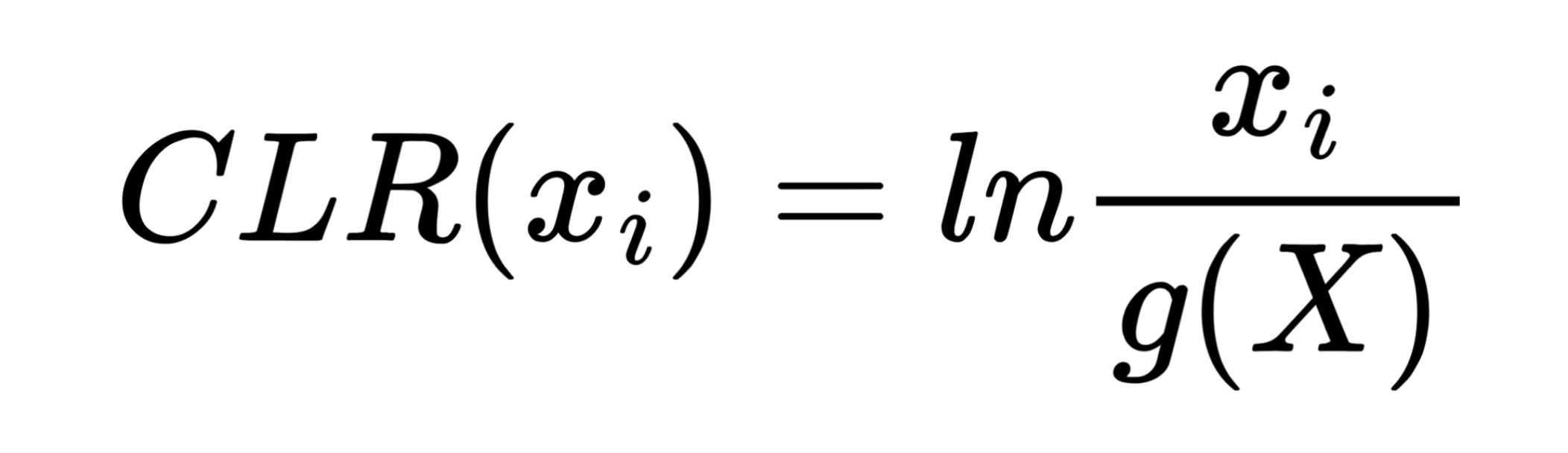
The first step in Neural network analysis was data transformation it is a crucial step to help machine learning algorithms properly learn patterns from the data. After literature study we concluded that Centered Log Ratio (CLR) is widely used for compositonal data which was the case for feature tables we were working on. We also split the dataset into train/validation (99 samples) and test (25 samples) to exclude human impact on test results.
Class reduction
We also wanted to check relevance of classes, to test that we had 3 settings which differed in number of classes. 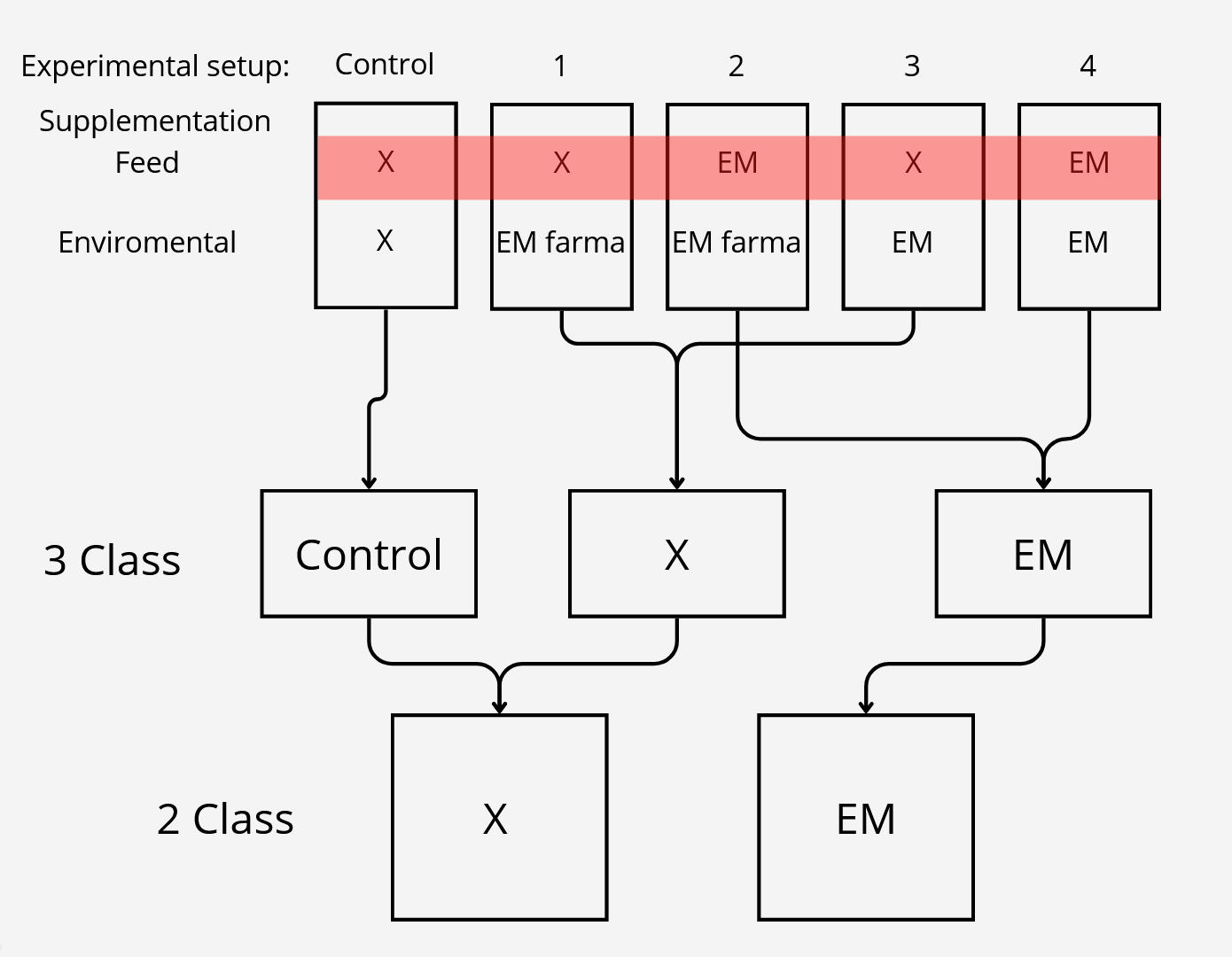
After the initial 5 class split which can be seen on the top, we came out with biological assumption that feed supplementation
should have much more impact on intestine microbiome than enviromental. On that basis we created 3 class split where control
setup was left untouched and experimental setups were divided based on feed supplementation, for the 2 class setting, class split was based only on feed supplementation.
Analysis pipeline
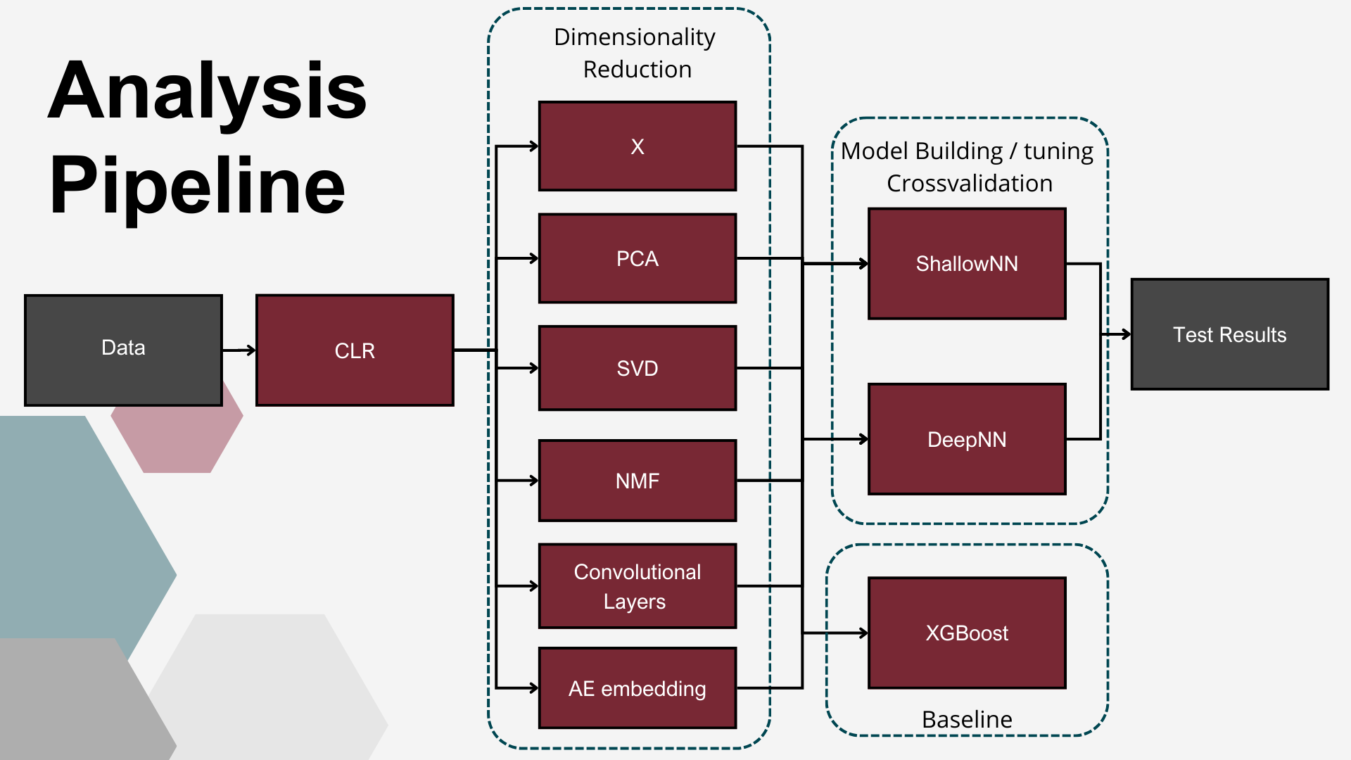
After data transformation, baseline setup and class split we compared 5 dimensionality reduction techniques with no reduction, and then used those reduced or not datasets for DL model building and tuning. For this step we performed 5 fold crosvalidation to achieve better undestanding of model performance. Here we trained models for 300 epochs. After the models were ready we tested them once on test dataset training for 500 epochs with early stopping to prevent overfitting.
Dimensionality reduction techniques (DRT)
In the study four approaches of reduced data representation were explored: One of them, Principal Component Analysis (PCA) (Pearson, 1901). To ensure consistency in the modeling pipeline, the PCA transformation was fitted on the training dataset and then applied to both the training and test datasets. PCA was first run iteratively with an increasing number of components, with a cumulative explained variance threshold of 90% as the initial target. Once the number of PCs required to meet this threshold was identified, a range of nearby component counts was also evaluated. These transformed datasets were then used as input for neural network classifiers to assess classification performance. Based on these results, the final number of principal components was selected to balance dimensionality reduction with classification accuracy.
The second DRT explored in this study was Singular Value Decomposition (SVD) (Golub & Reinsch, 1970). The transformation was fitted on the training dataset and then applied to both training and test sets. In the similar to PCA fashion, the number of components was determined based on variance threshold, and then nearby component counts were explored with regard to validation accuracy.
The third DRT applied in this study was Non-negative Matrix Factorization (NMF). Since NMF requires strictly non-negative input values, specifically for this approach the dataset was log-normalized with the addition of a small positive constant to avoid zero values. NMF was implemented using the scikit-learn package, with the maximum number of components set to 99. After factorization, all the components were used as the reduced representation of the dataset.
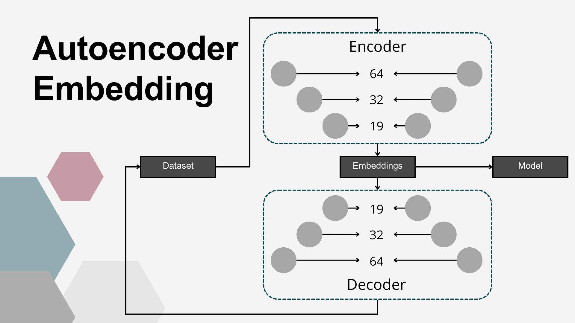
The fourth dimensionality reduction approach employed in this study was a DL–based embedding using AEs. Autoencoders are a class of unsupervised artificial neural networks designed to learn compressed, efficient representations of input data. An AE consists of two components: an encoder, which projects the input into a lower-dimensional latent space (embedding vector), and a decoder, which reconstructs the original input from this compressed representation. The network is trained to minimize the reconstruction error, ensuring that the learned embeddings capture the most relevant patterns in the data. In this study, the AE architecture was symmetrical, with both encoder and decoder composed of three fully connected layers using linear activation functions. The encoder comprised layers with 64, 32, and 19 nodes, resulting in a 19-dimensional embedding vector for each sample, producing an output matrix of shape n×19, where n=125 (the number of samples). Mean squared error (MSE) was used as the loss function, and the ADAM optimizer was applied during training, which continued until the loss function plateaued. Multiple AE configurations, varying in the number of layers and neurons per layer, were tested, with the final architecture selected based on best MSE results. The matrix of embeddings corresponding to the final AE model was used as the reduced representation of the input data set.
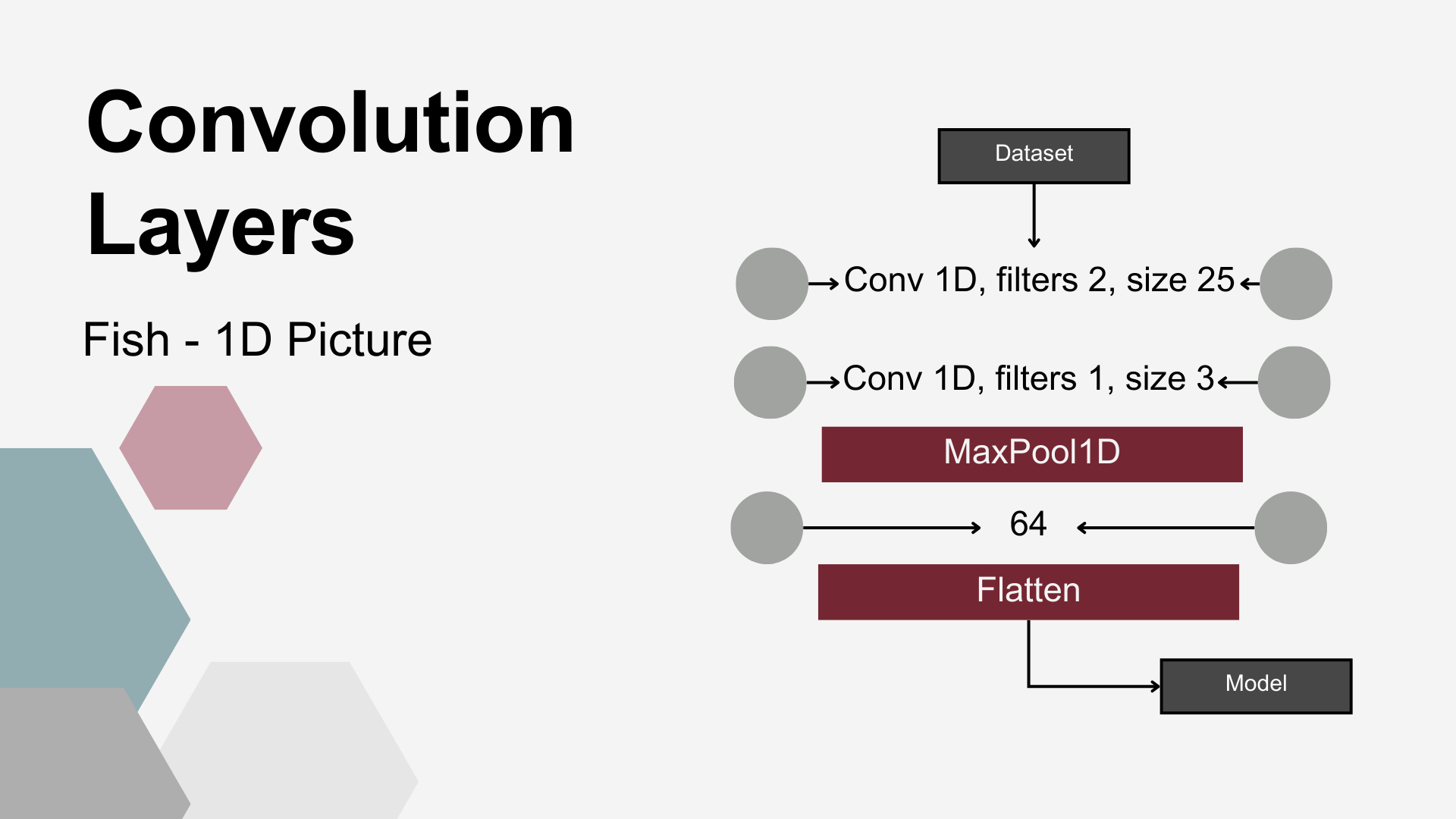
Fifth DRT utilized consisted of 1D convolution layers (Conv), most widely used in image analysis to extract structural patterns. The hypothesis underlying this study was that they might – similarly to image recognition – extract local abundance patterns from microbiome data. To enable pattern recognition, the input data was formatted such that each individual animal’s bacterial abundance represented a one-dimensional “image”. First, a 1-D convolutional layer was applied to the input data. This layer used two convolutional kernels, each with a kernel size of 25. The next layer was also a 1-D convolutional layer, utilizing a single kernel with a size of 3. Following the convolutional layers, a MaxPooling1D layer with a pool size of 4 was applied. This operation downsampled the feature maps, reducing dimensionality while emphasizing the most dominant local patterns. The subsequent layers consisted of a Dense layer with 64 units, followed by a Flatten layer, which reshaped the output into a one-dimensional vector suitable for further processing by the classification models.
Classifiers
Two Neural Netwok Architectures were employed as classifiers in this study, A Shallow (SNN) and Deep (DNN) Neural network,
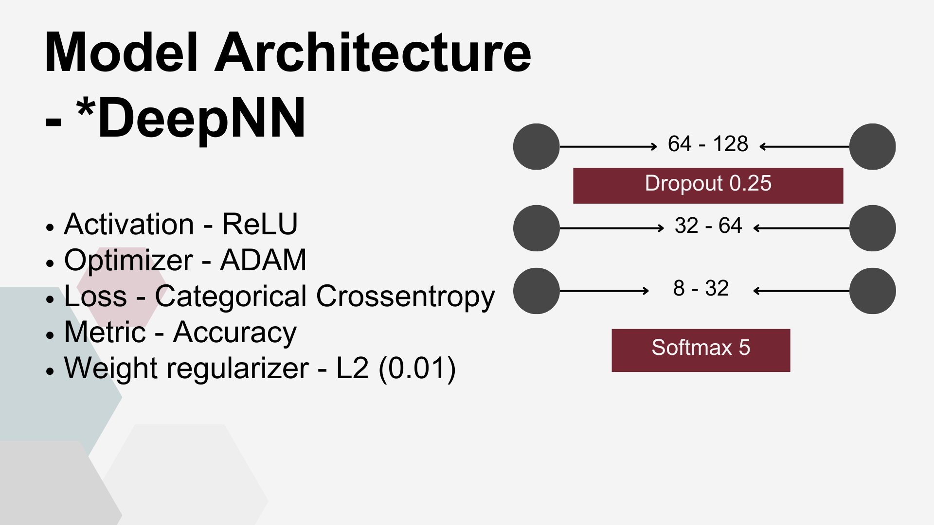
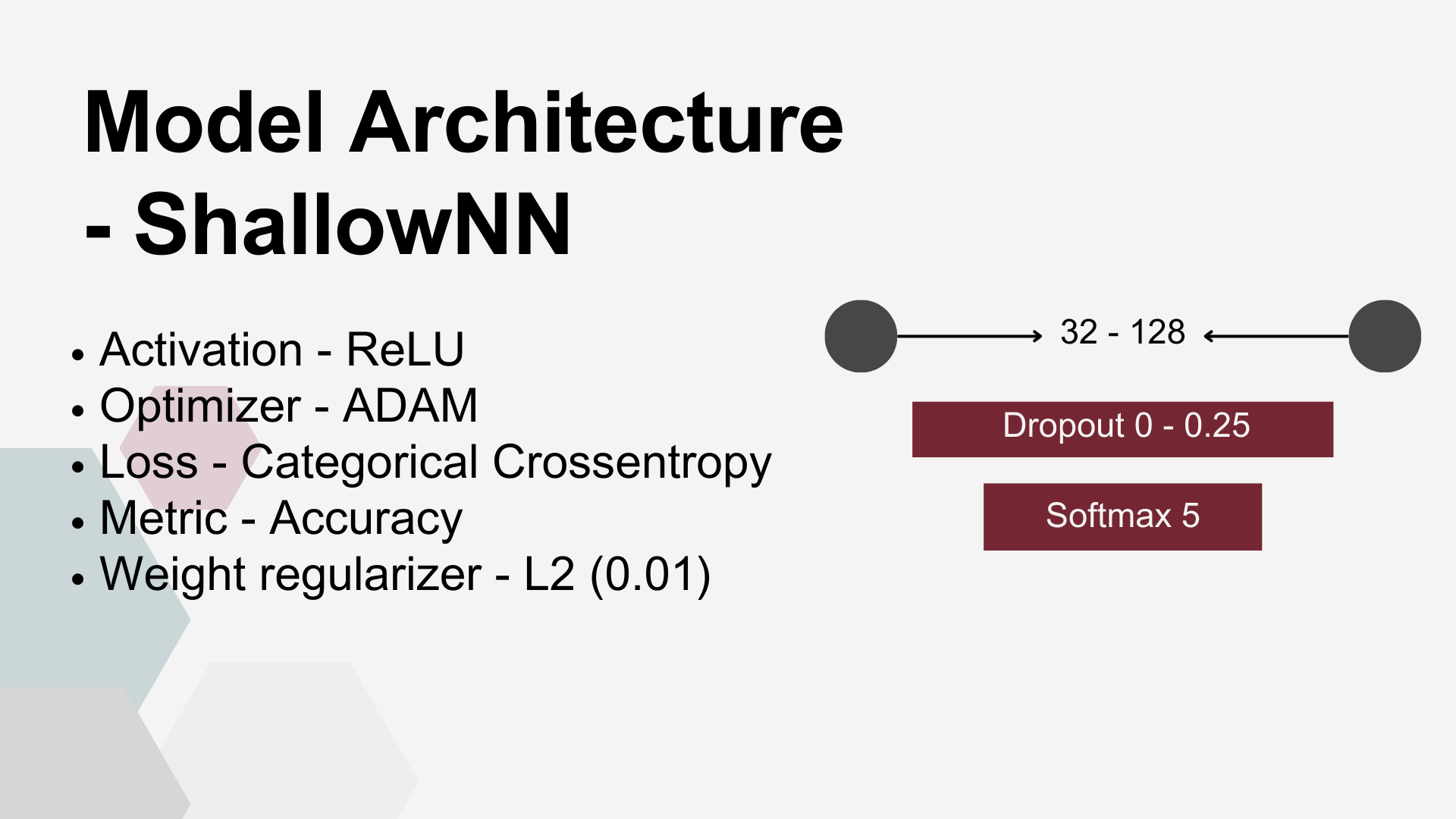
Both network architectures shared several key parameters: Rectified Linear Unit (ReLU) was the activation function for dense layers and smooth approximation of one-hot arg max (Softmax) was used for classification purposes at the output layer. Adaptive Moment Estimation (ADAM) was used to minimize the Categorical Cross entropy loss function. There were also common overfitting prevention measures applied to both architectures: weight regularizer L2 and Dropout Layers.
Deep FNN – a multi-layer model consisting of four dense layers with progressively decreasing node counts that dependent on DRT used, see table, followed by an output layer with nodes equal to the number of target classes (5, 3, or 2, depending on the scenario). A Dropout layer with a rate of 0.25 was placed after the first dense layer.
Shallow FNN – a minimal configuration designed to test the simplest viable architecture. It consisted of a single dense layer with a small number of nodes, usually close to the input dimensionality, directly connected to the classification output layer.
Additionally to establish robust baseline, XGBoost Algorythm was used.
Results DL
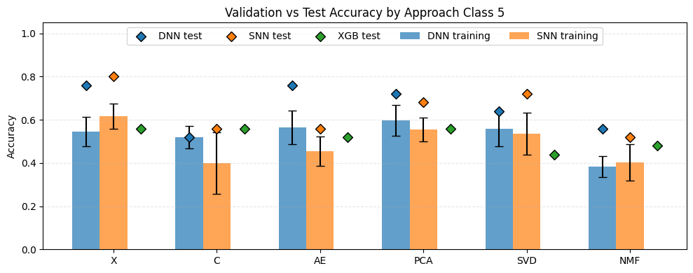
The plot above illustrates the results for the five-class classification task. The Y-axis represents the accuracy of the evaluated approaches, while the X-axis corresponds to the applied dimensionality reduction techniques. In this scenario, the expected accuracy for random class assignment is 0.2. Classifier types are indicated by colors: blue – Deep Neural Network (DNN), orange – Shallow Neural Network (SNN), and green – XGBoost. The bars represent the mean cross-validation accuracy, with whiskers indicating the standard deviation, while the points correspond to the test set results. A first observation is that, in general, test set results were higher than cross-validation results, and in most cases also higher than the baseline XGBoost performance. Furthermore, all evaluated models achieved accuracies exceeding the worst-case random baseline of 0.2. Among the neural network models, the highest test accuracy was observed for X-SNN (0.80), followed closely by X-DNN and AE-DNN (both 0.76). The lowest test accuracy was obtained for NMF-SNN and C-DNN (0.52), followed by AE-SNN, C-SNN, and NMF-DNN (all 0.56). Regarding the baseline XGBoost classifier, the worst performance was observed when the input data were reduced using NMF (0.44). The best performance was achieved when PCA or X features were used (both 0.56), although the differences between these configurations were not substantial.
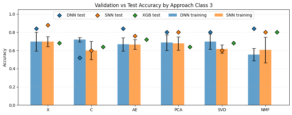
The plot above presents the results for the three-class classification task. Compared with the five-class scenario, a general increase in accuracy can be observed across most approaches. The lowest performance was observed for C-DNN (0.52) and C-SNN as well as SVD-SNN (0.60). All three of these models performed worse than the corresponding XGBoost classifiers applied to the same dimensionality reduction techniques, where XGBoost achieved an accuracy of 0.64. The highest accuracy was obtained for X-SNN (0.88). This was followed by X-DNN, NMF-DNN, and AE-DNN, each achieving an accuracy of 0.84. For the XGBoost baseline, the best performance was observed when the input data were reduced using NMF, reaching an accuracy of 0.80.
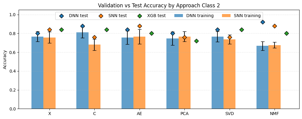
The plot above presents the results for the two-class classification task. Overall, the models achieved higher accuracies compared to the multi-class scenarios. The best performance was obtained for NMF-DNN, achieving an accuracy of 0.92. This was followed by C-DNN as well as NMF-SNN and AE-SNN, each reaching an accuracy of 0.88. The lowest performance among the evaluated neural network models was observed for PCA-SNN, SVD-SNN, and C-SNN, all with an accuracy of 0.76. Cross-validation results were generally consistent with the test results and did not differ substantially, with the exception of NMF-based models, which showed notably lower validation scores. The XGBoost baseline achieved accuracies ranging from 0.84 for C, SVD, and X representations to 0.72 for PCA-reduced data.
Simulation Study
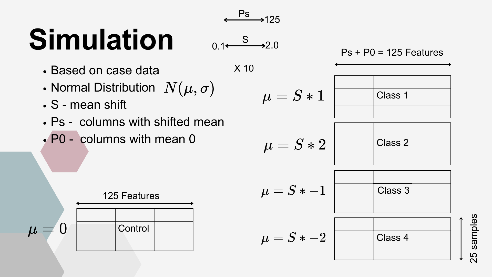
To assess properties of the proposed classification and anomaly detection approaches, a simulation study was conducted. The simulated data were based on the CLR-transformed original dataset and retained a similar structure (125 × 125) consisting of five classes.
In the first step, a standard deviation vector (V) was obtained from the original control group. This vector was subsequently permuted. The simulated control dataset was then generated by drawing 125 features for 25 samples, where each feature was sampled from a normal distribution N(0,Vi).
The simulation of experimental sets incorporated a parameter controlling the magnitude of the mean shift (S). Each simulated experimental set consisted of P0 features drawn from the same distribution as the control group, N(0,Vi), representing bacterial families not significantly affected by supplementation. The remaining features (Ps) represented bacterial families influenced by supplementation and were generated as follows:
- Class 1: N(S×1,Vi)
- Class 2: N(S×2,Vi)
- Class 3: N(−S×1,Vi)
- Class 4: N(−S×2,Vi)
Each class consisted of 25 samples, and the total number of features satisfied the condition P0+Ps=125. This design allowed control over the degree of separation between the control and experimental classes, enabling evaluation of the classification performance of the tested methodologies.
Simulations were performed separately for each analytical approach. For simulation, all the parameters like model architecture, number of components chosen for representation or size of latent space were kept the same as for case study. Each simulation scenario was repeated 10 times for every parameter combination. The number of affected features (Ps) ranged from 5 to 125 with a step size of 5, while the mean shift parameter (S) ranged from 0.1 to 2.0 with a step size of 0.1. Performance metrics were averaged across the repeated simulations.
Simulation Study Results
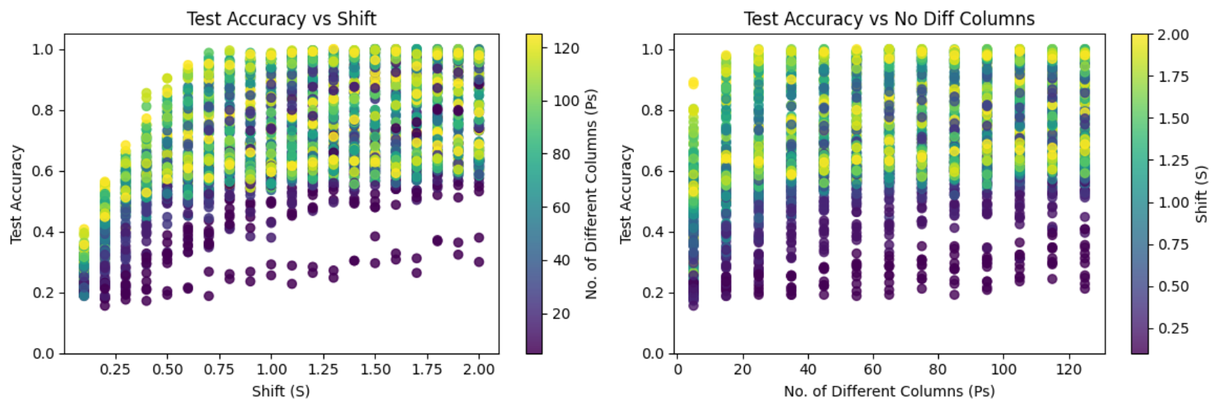
In the plots aggregated across all approaches, the left panel illustrates the relationship between accuracy and the shift parameter (S). A positive relationship can be observed up to approximately S = 0.75, after which relation begins to plateau, as accuracy approaches 1.0. In contrast, the right panel, which shows the relationship between accuracy and the number of affected features (Ps), does not exhibit a strong dependency. Accuracy remains relatively stable across most values of Ps, with only a slight decrease observed when the number of affected features is very small (Ps = 5).
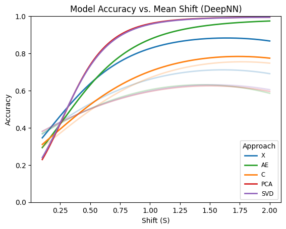
The plot above shows fitted quadratic polynomial regression curves describing the relationship between accuracy and the mean shift parameter (S) for each approach separately. Deep learning–based approaches are highlighted. Among the evaluated methods, PCA and SVD demonstrate clearly superior and very similar performance compared with the remaining approaches. These are followed by the autoencoder (AE) approach, while no dimensionality reduction (X) performs slightly worse. The convolution-based approach exhibits the lowest performance among the deep models. Overall, deep models substantially outperform their shallow counterparts across most dimensionality reduction techniques. For shallow models, however, the trend differs. In this case, the convolution-based representation achieves the best performance, followed by the no-reduction approach, while PCA, SVD, and AE show comparatively lower performance.
Comparative DL architectures Conclusions
- An overall increase in classification accuracy after class reduction was observed. This may be attributed either to a more biologically coherent representation of the classes or simply to the reduced number of possible misclassifications in problems with fewer categories.
- It is difficult to identify a clear best-performing approach in the case study, as the results varied considerably depending on the class split. This variability may be explained by the similar characteristics of the applied dimensionality reduction techniques or by the instability of neural network models when trained on small datasets.
- In the majority of evaluated scenarios, neural network models achieved higher performance than the XGBoost baseline, suggesting that deep learning approaches may represent a promising direction for microbial classification tasks.
- Regularization and dropout played an important role in mitigating overfitting. Given the small sample size and the zero-inflated nature of the microbiome dataset, overfitting was a major concern. The use of dropout (removing 25% of connections) and L2 weight regularization (0.01) likely contributed to more stable training, particularly for feed-forward neural network (FNN) models, enabling improved performance on the test set.
- The simulation study further demonstrated that:
- The magnitude of abundance differences (mean shift) had a substantially greater impact on classification performance than the number of affected features (bacterial families).
- Deep neural network (DNN) models consistently achieved higher performance than shallow models.
- Among the evaluated DNN architectures, PCA-DNN and SVD-DNN achieved the best results, whereas the convolution-based approach showed the lowest performance.
Measuring Feature Importance
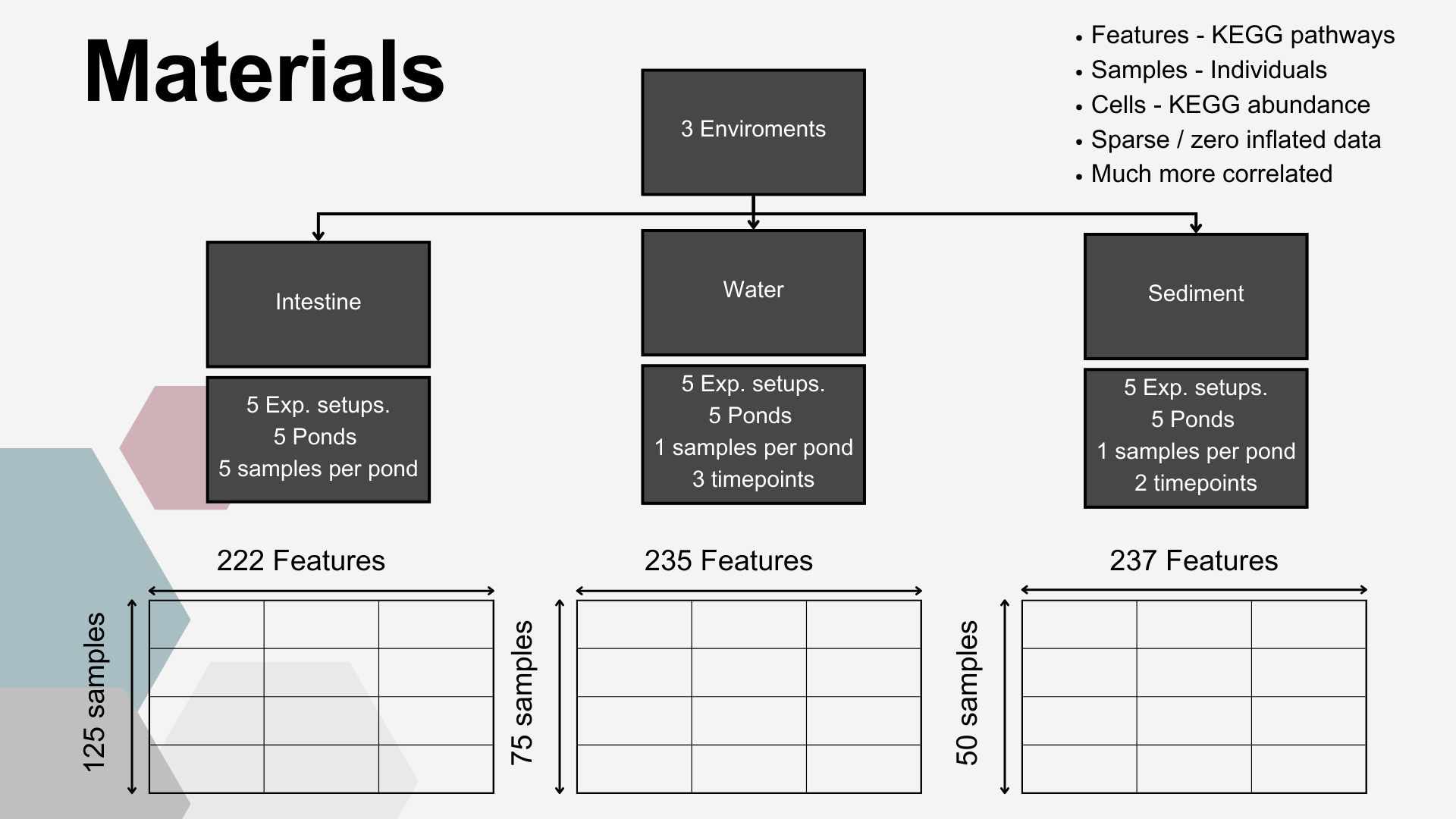
For this part of the analysis, KEGG pathway data were utilized. These data were obtained by first assigning KEGG orthologs to the taxonomically annotated dataset using PICRUSt2. Subsequently, KEGG pathways were mapped to the predicted orthologs using ggpicrust2.
Data from all enviroments (Intestine, Water and Sediment) was utilised for this part. Those Envirometns differed signifincatly in terms of number of samples, timepoints at which those samples were collected, number of KEGG pathways identified.
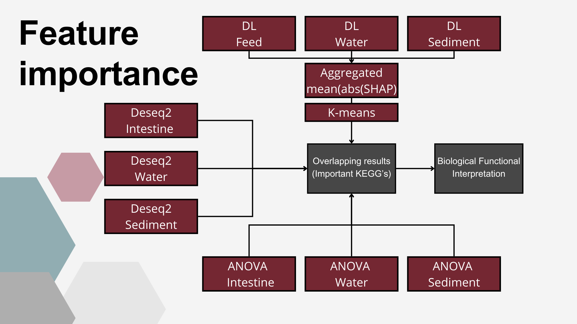
In each enviroment, level at which KEGG pathways were affected by supplementation was measured in three ways; ANOVA, Deseq2 and by DL-SHAP values.
DL – based feature importance
In the next step, deep learning architectures based on Dense Neural Networks (DNNs) were applied to classify ponds based on KEGG pathway abundance patterns observed in water, sediment, and fish gut samples, respectively. A common general architecture (visualized in Figure below) was used, while the hyperparameter configurations—including the number of nodes, dropout rate, kernel regularization strength, and learning rate—were optimized separately for each environment using Ray Tune.
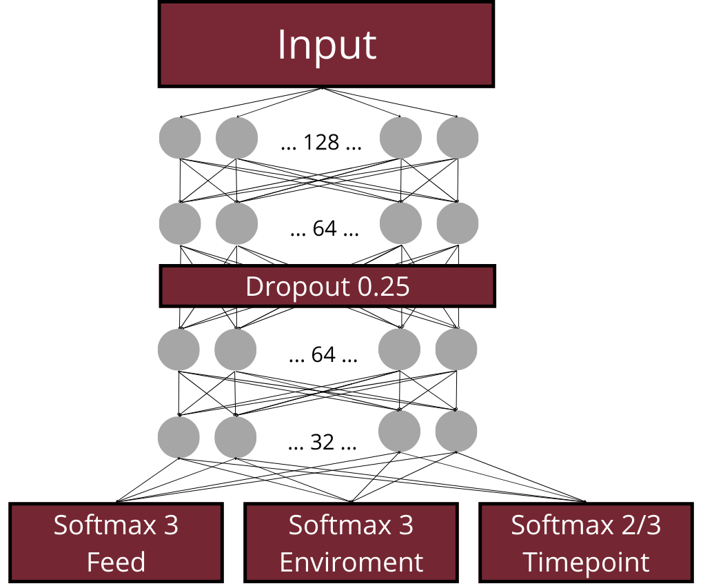
The models were trained to perform several classification tasks: (i) identification of the type of feed supplementation, (ii) identification of the type of environmental supplementation, and, for the water and sediment datasets, (iii) prediction of the sampling time point. Among the tested architectures, the best-performing configuration was selected based on validation performance. This model was subsequently retrained using the combined training and validation datasets and evaluated on the independent test set. Training continued until the loss function failed to improve for 100 consecutive epochs, after which the weights from the best-performing epoch were restored using an early stopping callback. At the output stage, the network contained parallel softmax output layers responsible for classifying feed supplementation type and environmental supplementation type. For the water and sediment datasets, an additional softmax output layer was included to perform sampling time point classification.
To assess the contribution of individual KEGG pathways to the DL-based classification, i.e. to differentiation between experimental setups, SHapley Additive exPlanations (SHAP) values (Shapley, 1988) were computed using the SHAP package (Lundberg and Lee, 2017). A kernel explainer was constructed based on the best DL model for each of possible classification outputs in the training/validation set and SHAP values were calculated for each KEGG. The final importance metric was calculated as the mean of absolute SHAP values calculated for each classification output. In the next step, the 1D K-means algorithm (Lloyd, 1957; MacQueen, 1967) was applied to cluster the mean SHAP values into groups representing KEGG pathways important and non-important for classification, which is biologically equivalent to pathways that were markedly altered by the EM supplementation.
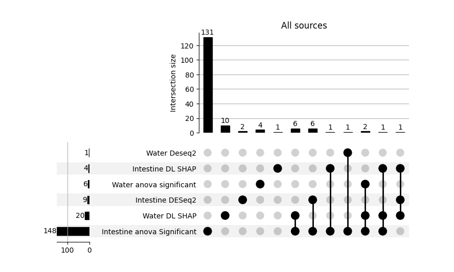
Feature importance results
For the intestinal dataset, the model achieved an accuracy of 0.48 for environmental supplementation classification and 0.64 for feed supplementation classification. For the water dataset, the model achieved high accuracy for sampling time point prediction (0.87). However, the performance for feed supplementation and environmental supplementation classification was much lower, reaching approximately 0.40, which is close to random classification performance. For the sediment dataset, the results suggest that the model did not train effectively, likely due to the limited sample size (n = 50). The accuracy did not exceed 0.50 for any of the classification tasks. Consequently, the sediment dataset was excluded from subsequent feature importance analyses. K-means clustering into important and non important features revealed 4 intestine and 20 water kegg pathways that were significantly impacted by EM supplementation. Those were then combined with other sources of feature importance in order to determine overlap between those and identify potentially meaningfull shifts in microbial structure.