Bioinformatic modelling of the impact of probiotic supplementation on microbiomes of breeding ponds and of digestive tract of the Common carp (Cyprinus carpio)
Title: Bioinformatic modelling of the impact of probiotic supplementation on microbiomes of breeding ponds and of digestive tract of the Common carp (Cyprinus carpio)
Key investigators: Joanna Szyda, Tomasz Suchocki, Anita Brzoza, Magda Mielczarek, Dawid Słomian, Michalina Jakimowicz
Students involved: Piotr Hajduk, Laura Jarosz, Marek Sztuka
Period of work: 2022-2026
Funded: National Science Centre
Introduction
In recent years, there is great interest in the use of effective microorganisms as probiotic supplementation in aquaculture to improve water quality, inhibit pathogens, and promote the growth of farmed fish. The use of probiotics, which control pathogens through a variety of mechanisms is viewed as an alternative to antibiotics and has become a major field in the development of aquaculture. Considering the potential benefits of adding probiotics, many farmers have recently been using commercially available products in their fish farms.
Although the practical efficacy of probiotic products in aquaculture has been extensively studied, there is a shortage of research related to practical, on-farm (i.e. not experimental) application of probiotic products in the Common carp (Cyprinus carpio) breeding. Especially when probiotics are implemented as a mixture of effective microorganism communities and not as a particular bacteria species.
This study aims to investigate the practical on-farm application of probiotics in Common carp (Cyprinus carpio) breeding, particularly when implemented as a mixture of effective microorganism communities. Probiotics have gained attention in aquaculture as an alternative to antibiotics, with the potential to improve water quality, inhibit pathogens, and promote fish growth. However, there is a lack of research on the practical application of probiotics in Common carp breeding. The study will assess the impact of probiotic supplementation on the water, sediment, and fish intestinal microbiota diversity in earthen ponds, which simulate practical fish breeding conditions. The study will also analyze the differences in water metatranscriptome compositions, with two major factors considered: (i) probiotic supplementation of water, and (ii) probiotic supplementation of feed. The findings of this study will contribute to the understanding of the practical application of probiotics in Common carp breeding and provide insights into the potential benefits of using probiotics in aquaculture.
Hypoteses
1. Microbiota diversity of water, sediment and fish intestinum can be altered by probiotic supplementation of water/feed.
2. Microbiota dynamics of water, sediment and fish intestinum differs between different probiotic supplements of water/feed.
3. There exists a correlation between the degree of microbiota diversity in water, sediment and in fish intestinum.
4. The abundance of particular taxonomical units does not change linearly in time.
5. Water metabolic activity expressed by water metatranscriptome varies between different probiotic supplements of water/feed.
Progress
The experimental part of the project was carried out during its first year at the Golysz experimental station, belonging to the Polish Academy of Sciences Institute of Ichthyobiology and Aquaculture. The complex of experimental aquaculture ponds comprised 32 equal-sized ponds of 600 m2 area. All ponds had individual water supply from the Vistula river, which guaranteed uniform physicochemical characteristics of supplied water. The whole experiment was carried out within one full fish production season. During the experiment, all ponds were stocked with the Common carp (Cyprinus carpio) hatchling applying a density of 30,000 larvae per hectare. Two most commonly commercially available probiotic water supplements, as well as one commercially available feed supplement, were tested in the experiment. The whole experimental setup involved 25 experimental ponds, from which 5 ponds were used as a control.


From each pond, 5 samples of water and sediment were collected 3 times during the experiment: (1) in the first month of the experiment, (2) after 2 months, and (3) in the last month of the experiment. In the last month of the experiment, fish intestinal samples were also collected from 5 individuals per pond, as well as one water sample per pond collected for metatranscriptome analysis. DNA was isolated and amplified for sequencing of selected hypervariable regions of the 16S rRNA gene from each sample intended for metagenomic analysis. Moreover, during the course of the experiment, regular measurements of water physicochemical parameters (temperature, pH, O2 concentration, nitrite, nitrate, ammonia, phosphorus) were performed to collect metadata describing water quality. At the beginning and the end of the experiment, sediment samples from all ponds were collected to analyze potential differences in sludge accumulation between ponds.


Sequencing
The sequencing process went well. The number of sequences for water samples can be found below.

The plots below express the quality of raw 16S rRNA data.


Analysis
For the 16s RNA analysis, the QIIME2 software was used. First of all, adapter trimming eliminated non-biological information was done. A quality threshold of 30 was applied to exclude sequences with a quality score below that threshold. Moreover, sequences shorter than 200 nucleotides were removed. Paired ends were merged with specific thresholds, maintaining sequence length consistency within 16S regions. The denoising step was performed, which produced Amplicon Sequence Variants (ASVs), distinguishing single-nucleotide differing sequences—an advancement over Operational Taxonomic Unit (OTU) tables. These tables were then used to determine the microbial composition of the samples. After that taxonomic assignment was performed. The alpha diversity metric was computed based on the taxonomic assignment. Furthermore, ANCOM was employed to conduct a differential abundance test for detecting alterations in the microbial composition between experimental groups.
The next step was to assign the ASV to Kyoto Encyclopedia of Genes and Genomes (KEGG) pathways. To achieve this, we used pictrus2 software to assign ASV to Kegg orthologs (KO), then KOs were used as an input to ggpicrust2 library (in R) that assign pathways based on KO’s. The last step in this part was to check if there are significant differences in the abundance of KEGG pathways between different design setups; this was done using Deseq2 package in R.
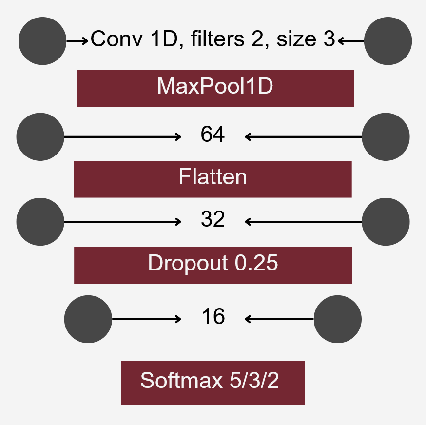
Neural Network Classification
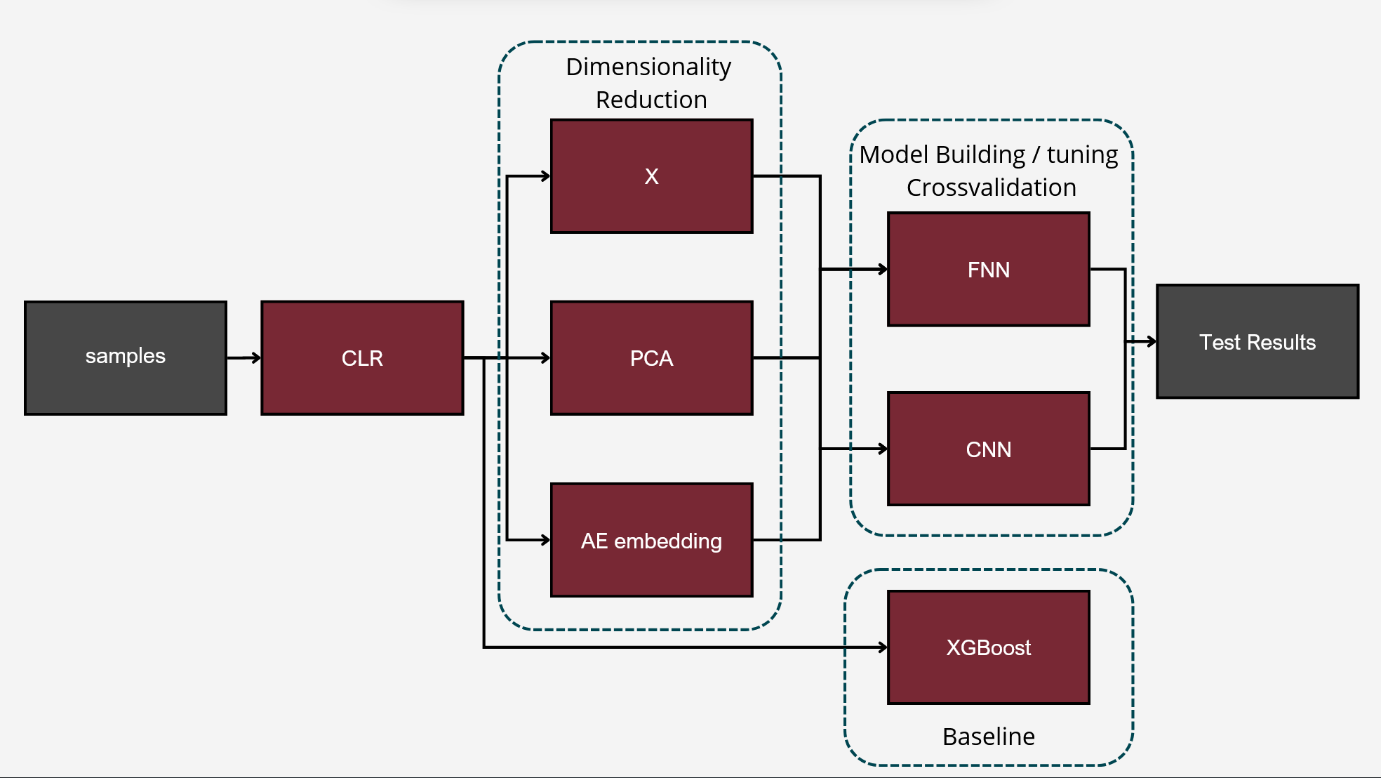
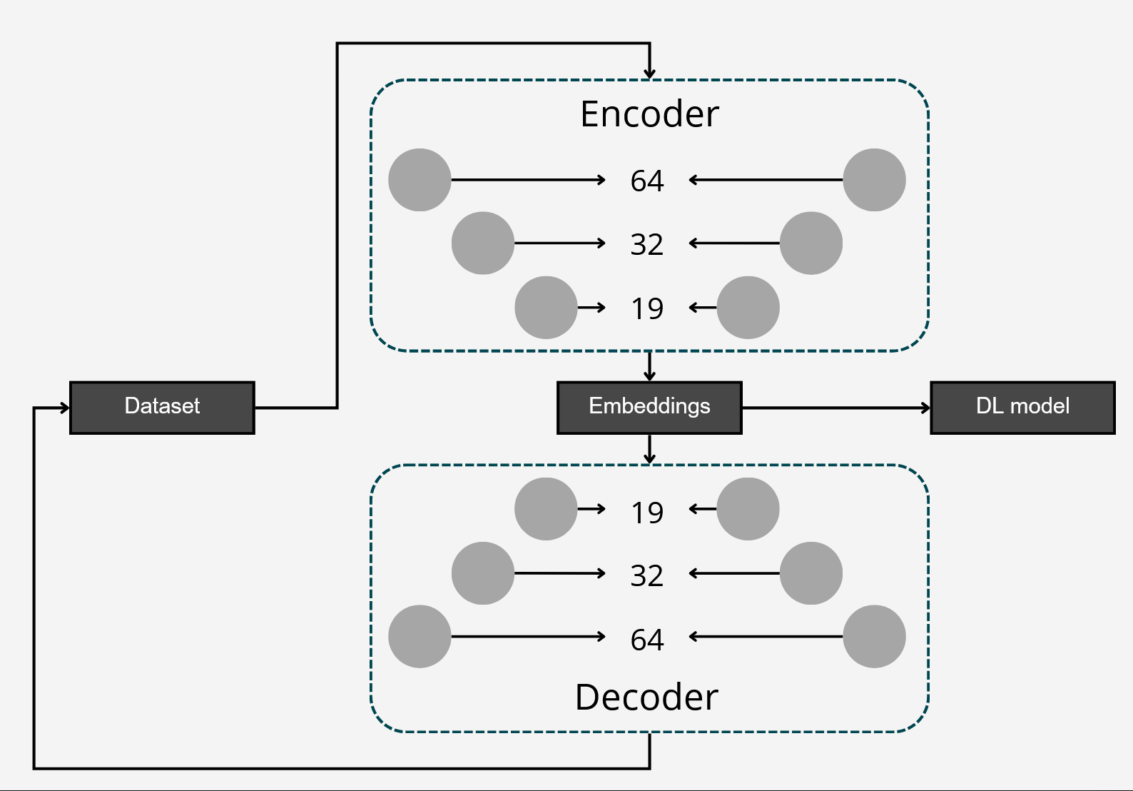
The model aimed to construct a neural network classifier using Keras under TensorFlow. The dataset consisted of feature tables representing the abundance of bacterial families in various individuals from different ponds. These tables were merged into a single dataset, including all bacterial families present in at least some individuals. Missing values were replaced with zeroes.
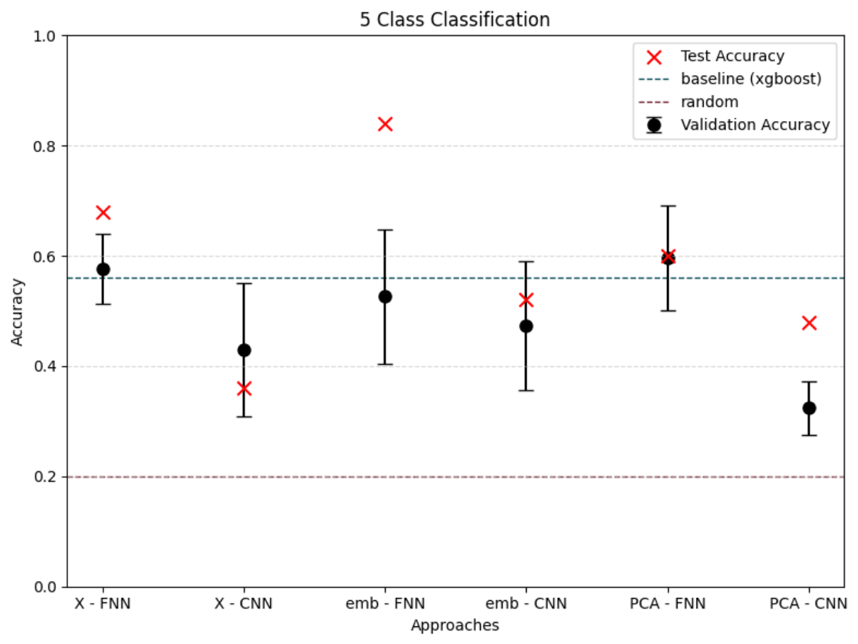
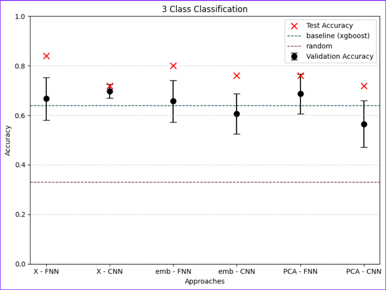
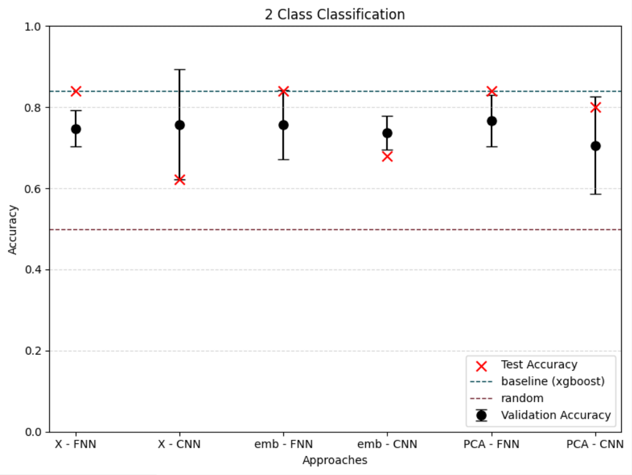
To differentiate microbiomes and classify individuals based on the probiotics they were fed, we tested and compared various deep learning methodologies. Specifically, we explored different dimensionality reduction techniques (PCA, autoencoder embeddings) and model architectures (FNN, CNN) to develop a deep learning classifier capable of performing this task.
For classification, the experimental setup (i.e., the type of probiotics fed to the individuals) was used as the class label, while the abundance of bacterial families served as predictors.
Accuracy was used as the primary evaluation metric. It was calculated on a binary basis, where each correctly classified experimental setup received a score of 1, and each misclassification received a 0. The final accuracy was determined by averaging these scores.
Data Transformation
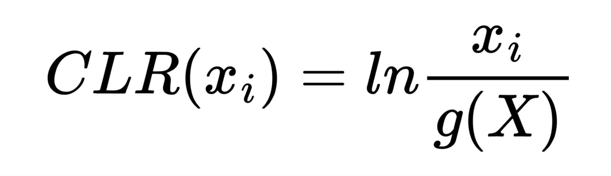
The first step in Neural network analysis was data transformation it is a crucial step to help machine learning algorithms properly learn patterns from the data. After literature study we concluded that Centered Log Ratio (CLR) is widely used for compositonal data which was the case for feature tables we were working on. We also split the dataset into train/validation (99 samples) and test (25 samples) to exclude human impact on test results.
Baseline
For the next step we wanted to setup baseline method to which we could compare our results, we had two of those first being random class assigning, for the second we wanted Machine Learning algorithm that is more robust than Neural Network with lesser number of tunable parameters. After literature study we settled on XGBoost with maximum depth of the tree 3. We trained it for 300 iterations.
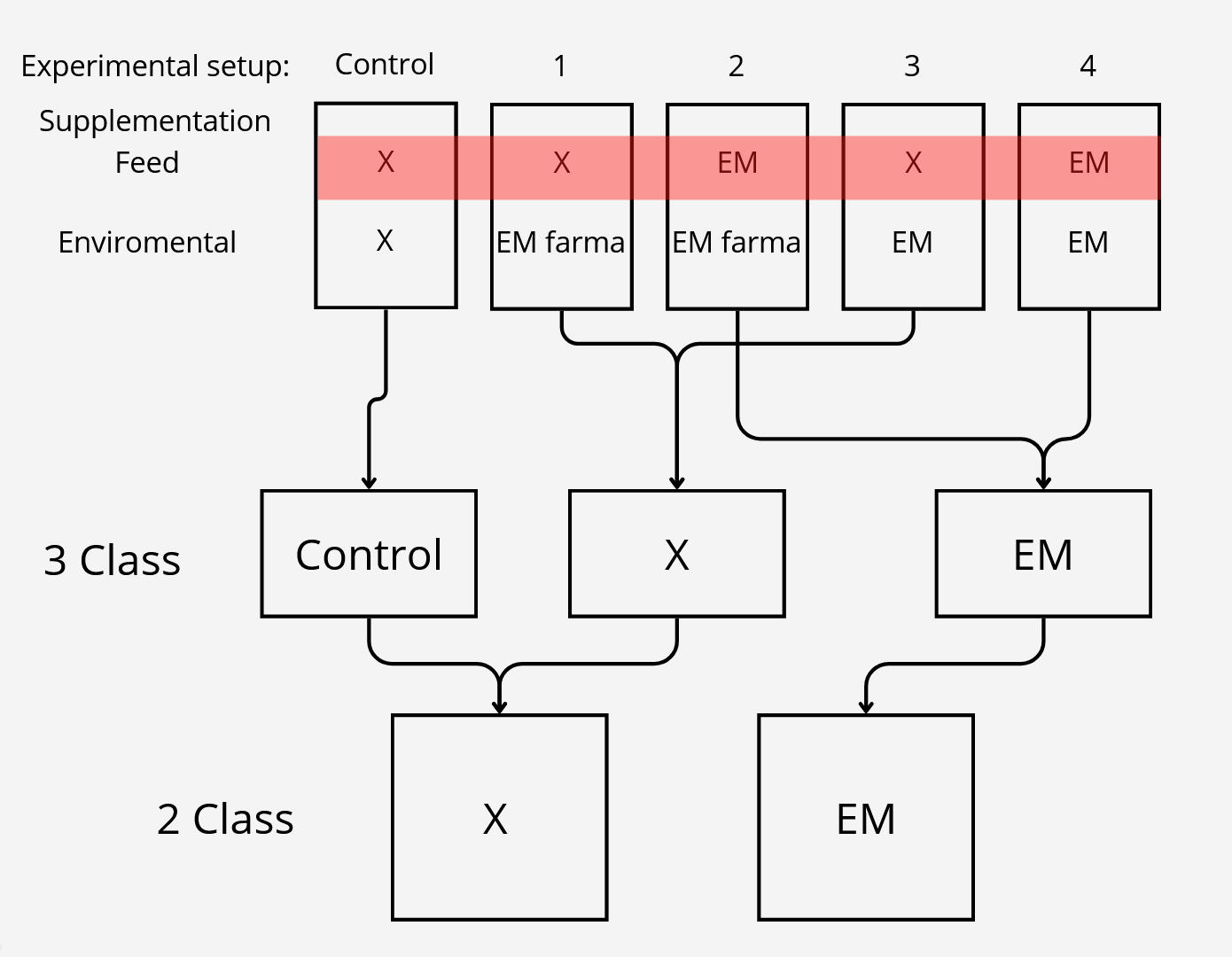
Class reduction
We also wanted to check relevance of classes, to test that we had 3 settings which differed in number of classes.